A minor extension of the Rubin causal analysis model

Photo by fabio on Unsplash

The Rubin causal model is the conceptual foundation for counterfactual impact evaluation and provides a powerful framework for specifying the conditions under which an average outcome based on a sample will recover an unbiased estimate of the impact of an intervention. The model starts with a thought experiment that compares a universe in which an individual receives a treatment with a (mutually exclusive) universe in which an individual does not.

Y_i = Y_0i + (Y_1i – Y_0i)D_i

Y_i – Observed outcome for individual (subscript i)

Y_0i – Outcome for individual having not received treatment (0 = not received)

Y_1i – Outcome for individual having received treatment (1 = received)

D_i – Treatment allocation status: D = 1 treatment group, D= 0 not treated group

Treatment effect = (Y_1i – Y_0i) – outcome for individual if treated minus outcome for same individual if not treated

This model is then extended to look at the averages (expectations) of groups of people, some of whom have been treated and others who have not, a formulation which precisely identifies selection bias.

E[Y_i|D_i = 1] - E[Y_i|D_i = 0]

= (E[Y_1i| D_i = 1] - E[Y_0i| D_i = 1]) + (E[Y_0i| D_i = 1] - E[Y_0i| D_i = 0])

In this context, the ‘missing’ data, is the average outcomes for the treatment group if they had not been treated (E[Y_0i| D_i = 1]), and selection bias is given by the difference in outcomes for the people allocated to the treatment group if they hadn’t been treated versus the outcomes for the people allocated to the non-treatment group (E[Y_0i| D_i = 1] - E[Y_0i| D_i = 0]). This is clearer graphically than it is algebraically.

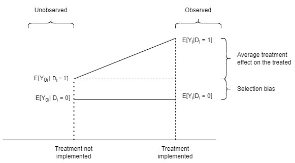
Though the graph makes the model clearer, it is unhelpful in one sense because moving from left to right is moving between two, mutually exclusive universes. It is not moving through time (ie ‘treatment implemented’ is not chronologically after ‘treatment not implemented’), but this can be easy to miss. However, this does indicate a way in which the model can be extended to include a time dimension, which graphically would mean changing the diagram from a 2D one to a 3D one by adding a z axis for time (algebraically adding a third subscript to indicate before and after). This means that the bias changes from a pure selection bias to a time and selection bias.

(E[Y_1i1| D_i = 1] - E[Y_0i1| D_i = 0])

= (E[Y_1i1| D_i = 1] - E[Y_0i1| D_i = 1])

+ {[(E[Y_1i1| D_i = 1] - E[Y_0i0| D_i = 1])]

- [(E[Y_0i1| D_i = 0] - E[Y_0i0| D_i = 0])}

This is a fairly unwieldy expression and more difficult to show graphically, but not that complicated to describe in words:

naive estimate (outcomes for treatment group having been treated - outcomes for non treatment group measured after the treatment period)

= impact (outcomes for treatment group having been treated - outcomes for treatment group if they hadn’t been treated measured after the treatment period)

+ time and selection bias

• outcomes for treatment group having been treated minus outcomes for treatment group measured before they were treated

• minus outcomes for non-treatment group measured after the treatment period minus outcomes for treatment group measured before the treatment period

Within this formulation, an RCT recovers an unbiased estimate of impact by assuming that random assignment ensures there is no difference in baseline outcomes for the those in treatment and non-treatment groups (E[Y_0i0| D_i = 1]) = E[Y_0i0| D_i = 0]) and that there is no change over time as a result of being allocated into the intervention or control groups (E[Y_0i1| D_i = 1]) = E[Y_0i1| D_i = 0]), ie that allocation alone doesn’t cause any difference in outcomes. This second assumption is less foregrounded in the literature but is a serious issue in RCTs because it is not hard to imagine, for example, that being allocated to the control group could either make people despondent or work harder (thinking about an RCT of an educational programme for instance).

In contrast, difference-in-differences techniques recover an unbiased estimate by assuming a parallel trend during the treatment period, ie that:

E[Y_1i1| D_i = 1] - E[Y_0i0| D_i = 1] = (E[Y_0i1| D_i = 0] - E[Y_0i0| D_i = 0]

Meaning that the unobserved outcome is:

E[Y_1i1| D_i = 1] = E[Y_0i0| D_i = 1])] + {[(E[Y_0i1| D_i = 0] - E[Y_0i0| D_i = 0])}

The same danger applies to difference-in-difference analysis as it does to an RCT, that a time bias could be introduced as a result of being in the intervention group. In one study I was involved in, the evaluation of the Drug System Changes Pilots, found that this is exactly what seemed to have happened in that policy context. The pilots were given additional ‘freedoms and flexibilities’ but the innovations they implemented were mostly things they could already have done. So the impact seemed to be primarily due to being part of a pilot rather than as a result of the ‘treatment’ (not having to follow the same rules as other areas).

One advantage of extending the Rubin causal model to include time is that the bias involved in simple before and after measurements can be specified using the same notation.

E[Y_1i1| D_i = 1] - E[Y_0i0| D_i = 1]

= (E[Y_1i1| D_i = 1] - E[Y_0i1| D_i = 1])

- (E[Y_0i1| D_i = 1] - E[Y_0i0| D_i = 1])

Graphically this looks very similar to the original graph above, except that the two two lines start a single baseline point and selection bias is replaced by time bias. If you assume there is no time bias, ie that outcomes don’t change over time in the absence of the intervention (E[Y_0i1| D_i = 1] = E[Y_0i0| D_i = 1]), then the substitution can be made into the left hand side of the equation and before and after measurement directly recovers an unbiased estimate of impact.

Translating this to the real world, there are circumstances when it is plausible to think that there is no change to outcomes over a period of time. For example, if a maths test on a particular topic was administered before and after a lesson on that topic or a measure of attitudes was administered before and after a brief (eg hour long) presentation on a subject, it would be plausible to think that the change was purely the result of the intervention. Though these situations are relatively rare in policy evaluation, they are worth bearing in mind and should not be dismissed simply because they involve an untestable assumption because all approaches to counterfactual evaluation involve untestable assumptions. The important point is to acknowledge the assumption and provide an argument and ideally some evidence why it is plausible.